How To Draw Shear Stress Distribution Diagram

Shear and Moment Diagrams – An Ultimate Guide

In this mail we're going to accept a wait at shear and moment diagrams in detail. Determining shear and moment diagrams is an essential skill for any engineer. Unfortunately it'south probably the one structural analysis skill most students struggle with most.

This is a problem. Without understanding the shear forces and bending moments developed in a structure you can't complete a design. Shear strength and bending moment diagrams tell the states nigh the underlying state of stress in the structure. So naturally they're the starting betoken in any design process.

Some other reason every graduating engineer needs to accept a solid grasp of shear forces and angle moments is because they're absolutely going to be tested in almost every graduate interview. The quickest way to tell a great CV writer from a great graduate engineer is to ask them to sketch a qualitative bending moment diagram for a given structure and load combination!

And then in this post we'll give you lot a thorough introduction to shear forces, angle moments and how to describe shear and moment diagrams. We won't be able to embrace everything in this 1 post but hopefully you lot'll attain the stop knowing more than than when you lot started! If you desire to do a deep dive to really boom downwardly this skill, you lot should have a await at my course, Mastering Shear Force and Bending Moment Diagrams [🎓 At present Complimentary FOR STUDENTS]. In it, we'll cover the fundamental theory and put it into exercise with plenty of worked examples.

In this post we'll cover…

Download the DegreeTutors Guide to Shear and Moment Diagrams eBook. 📓
Mastering Shear Force and Bending Moment Diagrams
- Your consummate roadmap to mastering these essential structural assay skills.
i.0 What is a Angle Moment?
two.0 What is a Shear Force?
3.0 Calculating Internal Shear Forces and Bending Moments
four.0 Building Shear and Moment Diagrams
- 4.i Finding the location of the maximum angle moment
v.0 Drawing Shear Force and Bending Moment Diagrams – An Example
- 5.one Video Tutorial
- five.2 Calculating the back up reactions
- v.3 Drawing the shear forcefulness diagram
- 5.iv Drawing the bending moment diagram
6.0 Relating Loading, Shear Forcefulness and Bending Moment
- 6.one Instance ane: Uniformly distributed loading
- 6.ii Instance ii: Bespeak forcefulness loading
- half dozen.3 Instance 3: Point moment loading
7.0 Another Instance
- 7.1 Setup and shear strength diagram
- seven.2 Building the bending moment diagram
- 7.3 Confirming maximum moment with calculus
Build your ain shear force and bending moment solver
Beam & Frame Analysis using the Straight Stiffness Method in Python
- Build a sophisticated structural analysis software tool that models beams and frames using Python.
Tutorial by:
Dr Seán Carroll

one.0 What is a Bending Moment?

Let's start with a basic question; what is a bending moment? To answer this nosotros need to consider what'southward happening internally in a construction under load. Consider a merely supported beam subject to a uniformly distorted load.

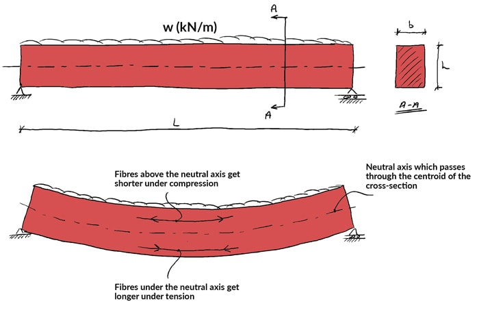
Shear-and-moment-diagrams-beam | DegreeTutors.com

The axle volition deflect under the load. In order for the axle to deflect equally shown, the fibres in the top of the axle must contract or get shorter. The fibres in the bottom of the axle must become longer.

We can say the top of the axle is in compression while the bottom is in tension (notice the direction of the arrows on the fibres in the deflected axle). Now, at some position in the depth of the beam, compression must plough into tension. There is a aeroplane in the beam where this transition between tension and compression occurs. This plane is called the neutral plane or sometimes the neutral axis.

Imagine taking a vertical cut through the beam at some distance $x$ along the axle. We can stand for the strain and stress variation throughout the depth of the beam with strain and stress distribution diagrams.

Shear-and-moment-diagrams-stresses | DegreeTutors.com

Call up, strain is only the change in length divided by the original length. In this case nosotros're considering the longitudinal strain or strain perpendicular (normal) to the cut face up.

Compression strains above the neutral axis be because the longitudinal fibres in the beam are getting shorter. Tensile strains occur in the lesser because the fibres are extending or getting longer.

We tin assume this beam is made of a linearly rubberband cloth and every bit such the stresses are linearly proportional to the strains. This only ways we demand to multiple the strain at some point in the axle by the Young's modulus (modulus of elasticity) to go the corresponding stress at that bespeak in the beam.

We know that if we multiply a stress past the area over which it acts, nosotros become the resultant strength on that surface area. The same is true for the stress acting on the cutting face of the beam. The compression stresses can be represented past a compression force (stress resultant) while the tensile stresses tin be replaced by an equivalent tensile force. So for case the compression forcefulness is given by,

(i) $\begin{equation*} F_c = \underbrace{\left[\sigma_t \times \frac{1}{2} \right]}_{\text{average stress}}\underbrace{\left[ b \times\frac{h}{2}\right]}_{\text{area}} \end{equation*}$

Shear-and-moment-diagrams-force-couple | DegreeTutors.com

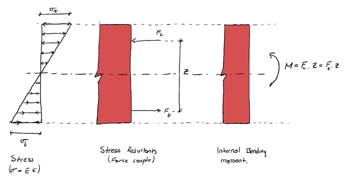
Equally a effect of the external loading on the construction and the deflection that this induces, nosotros end up with ii forces acting on the cut cross-section. These forces are:

equal in magnitude (must be to maintain force equilibrium)
parallel to each other (and perpendicular to the cutting face)
interim in reverse directions
separated by a distance or lever arm, $z$

Y'all might recognise this pair of forces equally forming a couple or moment $M$ .

(2) $\begin{equation*} M = F_c\times z = F_t\times z \end{equation*}$

💡 The internal bending moment $M$ , is the angle moment nosotros represent in a angle moment diagram. The bending moment diagram shows how $M$ (and therefore normal stress) varies across a structure.

If nosotros know the land of longitudinal or normal stress due to angle at a given section in a structure we can work out the respective bending moment.

However, more ofttimes information technology's the case that we know the value of the bending moment at a point and utilise this to work out the maximum values of normal stress at that location.

We do this using the Moment-Curvature equation a.k.a. the Engineer's Bending Equation…

(3) $\begin{equation*} \boxed{\sigma = \frac{-M\:y}{I}} \end{equation*}$

…which relates the stress, $\sigma$ at a distance $y$ from the neutral centrality, to the moment, $M$ . Where $I$ is the second moment of surface area for the cross-department.

Hopefully now y'all can conspicuously run into how angle moments arise;

external forces induce deflections
strains develop (which we meet at a larger scale every bit structural deflections)
where we have strains, we must accept stresses (retrieve Young's modulus)
these stresses, can be represented with their force resultants that ultimately course a couple or internal bending moment, $M$

2.0 What is a Shear Forcefulness?

We tin now turn our attention to shear forces and start with a simple definition;

💡 A shear force is any force interim perpendicularly to the longitudinal axis of the structure. We're typically interesting in internal shear forces that are the resultant of internal shear stresses developed in the structure.

Edifice on our discussion of bending moments, the shear force represented in the shear force diagram is as well the resultant of shear stresses acting at a given indicate in the structure. Consider the cut face of the axle discussed above.

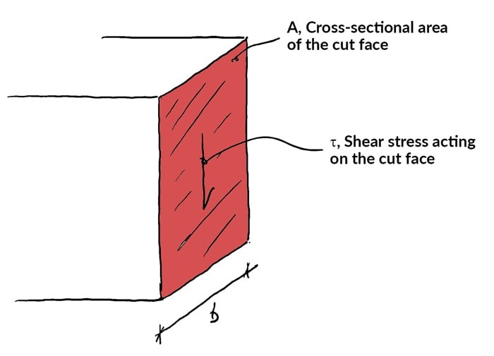
Shear-and-moment-diagrams-force-shear-stress | DegreeTutors.com

The shear stress, $\tau$ acting on this cutting face is evenly distributed across the width of the face up and acts parallel to the cut face. The average value of the shear stress, $\tau_{avg}$ is simply the shear strength at this point in the structure $V$ divided past the cantankerous-exclusive area over which it acts, $A$

(4) $\begin{equation*} \tau_{avg} = \frac{V}{A} \end{equation*}$

Withal, this is just the average value of the shear stress acting on the face. The shear stress actually varies parabolically through the depth of the department according to the following equation,

(5) $\begin{equation*} \tau = \frac{VQ}{Ib} \end{equation*}$

where, $Q$ is the first moment of expanse of the area to a higher place the level at which the shear stress is being determined, $I$ is the 2nd moment of area of the cantankerous-section and $b$ is the width of the department.

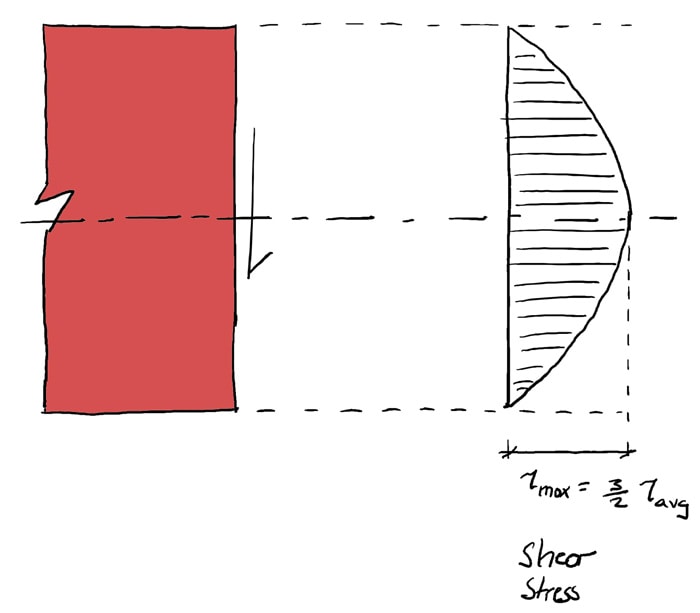
Shear-and-moment-diagrams-force-parabolic-shear-stress | DegreeTutors.com

We don't want to go as well far down the rabbit hole with shear stresses. For the purposes of this tutorial, all nosotros desire to practice is establish the link between the shear force we detect in the shear force diagram and the corresponding shear stress within the construction. Equations (four) and (five) do that for us.

three.0 Calculating Internal Shear Forces and Angle Moments

Up to this bespeak we've considered the link between the normal (angle) stress and associated bending moment and the shear stress and associated shear force. Based on this you should be comfortable with the idea that knowing the value of bending moment and shear force at a point are important for understanding the stresses in the structure at that point.

Now nosotros're going to consider the problem of calculating shear forces and bending moments not from the betoken of view of internal stresses but by considering equilibrium of the structure.

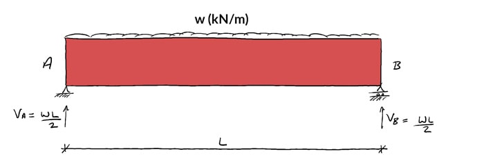
In reality, this is practically how we determine the shear force and bending moment at a point in the construction. Again, let's consider the simply supported axle from higher up, subject to a uniformly distributed load, $w$ kN/1000.

Simple statics tell us that if the axle is in a state of static equilibrium, the left and correct manus back up reactions are,

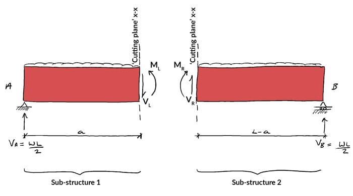
(six) $\begin{equation*} V_a = V_b = \frac{wL}{2} \end{equation*}$

Shear-and-moment-diagrams-beam-udl | DegreeTutors.com

If the structure is in a country of static equilibrium (which it is), and so whatsoever sub-structure or function of the structure must also be in a land of static equilibrium nether the stabilising activity of the internal stress resultants.

This is a cardinal indicate! Imagine taking a cut through the structure and separating information technology into 2 sub-structures. When we cutting the structure, we 'reveal' the internal stress resultants (bending moment and shear strength).

Shear-and-moment-diagrams-sub-structure | DegreeTutors.com

$M_L$ and $M_R$ are the internal bending moments on either side of the imaginary cut while $V_L$ and $V_R$ are the internal shear forces on either side of the imaginary cut.

💡 $M_R$ and $V_R$ stand for the influence of the left hand side of the structure (sub-structure 1) on the correct hand side of the structure (sub-construction 2) and vice versa.

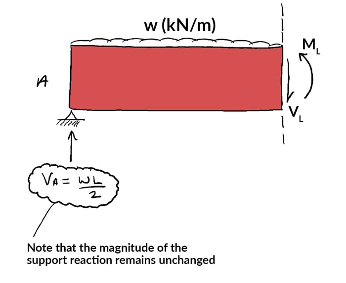
Nosotros've just said that each i of these sub-structures is stabilised past the influence of the internal angle moment and shear forcefulness revealed by the imaginary cuts.

This means, if we desire to find the value of internal bending moment or shear force at any point in a structure, we simply cut the construction at that point to expose the internal stress resultants ( $M$ and $V$ ). Then calculate what values they must have to ensure the sub-structure remains in equilibrium! For example the sub-structure below must remain in equilibrium under the combined influence of:

Shear-and-moment-diagrams-sub-structure-1 | DegreeTutors.com

This starts to make more than sense when we plug some numbers into an case. For the beam above, let's imagine it has a span $L=6$ m, applied loading of $w=10$ kN/m and imagine nosotros cut the axle at $a=2$ m from the left paw back up.

The left manus reaction, $V_A$ is,

(7) $\begin{equation*} V_A = \frac{w L}{2} = \frac{10\times 6}{2} = 30 \:\text{kN} \end{equation*}$

Now taking the sum of the moments almost the cut and assuming clockwise moments are positive,

(viii) $\begin{align*} &\sum M_{\text{cut}}=0\\ &(30\:\text{kN}\times 2\:\text{m}) - (10\:\text{kN/m}\times 2\text{m}\times 1\text{m}) -M_L=0\\ & \therefore \: M_L = 40 \:\text{kNm} \end{align*}$

Then, the internal bending moment required to maintain moment equilibrium of the sub-structure is $40$ kNm. Similarly, if we accept the sum of the vertical forces acting on the sub-structure, this would yield $V_L = 10$ kN.

4.0 Building Shear and Moment Diagrams

In the final section we worked out how to evaluate the internal shear strength and bending moment at a discrete location using imaginary cuts. But to draw a shear force and bending moment diagram, we need to know how these values change beyond the structure.

What we actually want is an equation that tells united states the value of the shear strength and angle moment as a function of $x$ . Where $x$ is the position along the beam. Consider making an imaginary cutting, just like above, except now we can make the cut at a distance $x$ forth the beam.

Now the internal shear forcefulness and angle moment revealed by the cut are functions of $x$ , the cutting position. Here, we'll determine an expression for $M(x)$ . But the procedure is exactly the same to decide $V(x)$ .

Shear-and-moment-diagrams-BMD | DegreeTutors.com

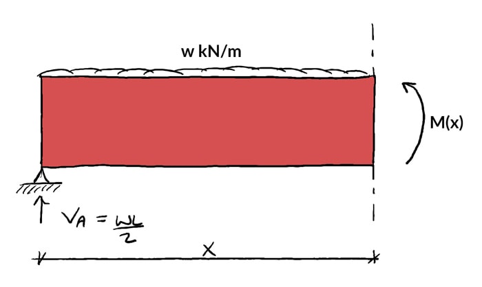
Taking the sum of the moments about the cut and over again bold clockwise moments are positive,

(nine) $\begin{equation*} \sum M_{\text{cut}}=0 \end{equation*}$

(10) $\begin{equation*} \frac{wL}{2}x - w x \frac{x}{2}-M(x) &= 0\\ \end{equation*}$

(xi) $\begin{equation*} M(x) &= \frac{wLx}{2} - \frac{wx^2}{2}\\ \end{equation*}$

(12) $\begin{equation*} M(x) &= \frac{wx}{2}(L-x) \end{equation*}$

At present we can apply equation (12) to determine the value of the internal bending moment for any value of $x$ along the beam. Plotting the bending moment diagram is but a matter of plotting the equation.

4.1 Finding the location of the maximum bending moment

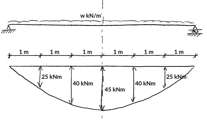
In the instance above, the structure and loading is symmetrical then it's pretty like shooting fish in a barrel to recognise the location of the maximum moment and then afterwards to evaluate it.

Yet this may not always be the case. So it's helpful to take a technique to identify the location of the maximum moment without needing to plot the total angle moment diagram.

In this example, the angle moment for the whole construction is described past a single equation…equation (12). You might call back from basic calculus that to place the location of the maximum bespeak in a function nosotros merely differentiate the function to get the equation for the gradient. And then it's only a matter of setting this function equal to zero and solving for x.

In other words, at the location of the maximum bending moment, the slope of the angle moment diagram is zero. So we just need to solve for this location. Once we have the location we can evaluate the angle moment using equation (12).

So, to demonstrate let's first evaluate the differential of equation (12),

(13) $\begin{equation*} \frac{\mathrm{d}}{\mathrm{d}x} M(x) = \frac{wL}{2} - wx \end{equation*}$

Think, equation (13) represents the gradient of the bending moment diagram. And then we now let it equal to zero and solve for $x$ .

(14) $\begin{equation*} \frac{wL}{2} - wx = 0 \end{equation*}$

(15) $\begin{equation*} \therefore x=\frac{L}{2} \end{equation*}$

Surprise surprise, the bending moment is a maximum at the mid-span, $x=L/2$ . Now we can evaluate equation (12) at $x=L/2 = 3$ m.

(16) $\begin{equation*} M(x=L/2) = \frac{wL^2}{4} - \frac{WL^2}{8} \end{equation*}$

(17) $\begin{equation*} \therefore M_{\text{max}} = \frac{wL^2}{8} = \frac{10\times 6^2}{8} = 45 \:\text{kNm} \end{equation*}$

There we have it; the location and magnitude of the maximum angle moment in this merely supported beam, all with some basic calculus.

5.0 Drawing Shear Strength and Bending Moment Diagrams – An Instance

Now that we have a grasp of the fundamentals, let's see how information technology all ties together with a bigger more complex worked example. This example is an excerpt from this class. Just a quick heads up, if you're new to shear force and bending moment diagrams, this question might be a bit of a claiming. If you become a bit lost with this case, it might be worth your time taking a look at this DegreeTutors form. Information technology's aimed at bringing you from scratch all the manner upwards to being comfortable analysing complex shear and moment diagrams.

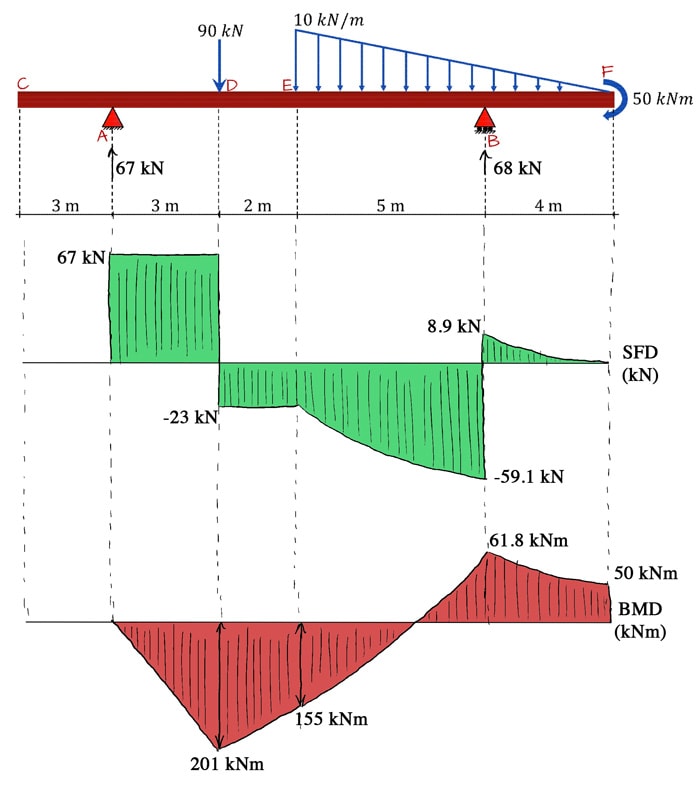
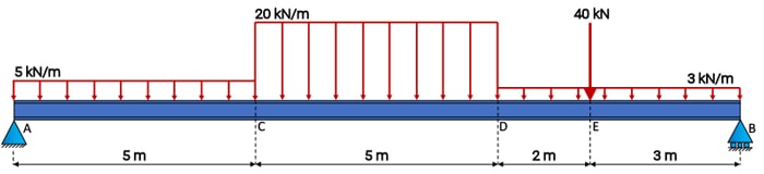
Ok, let'due south become on with it. We want to determine the shear force and bending moment diagrams for the following but supported beam.

Shear-and-moment-diagrams-example-question| DegreeTutors.com

You can continue reading through the solution below…or if you prefer video, you lot can sentry me walk through the solution here.

5.1 Video Tutorial

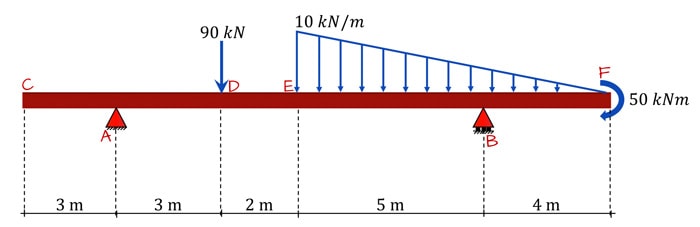
5.2 Computing the support reactions

The first step in analysing any statically determinate structure is working out the back up reactions. We can kick-off by taking the sum of the moments about betoken A, to determine the unknown vertical reaction at B, $V_B$ ,

(eighteen) $\begin{equation*} \sum M_{\text{A}}=0\:\:\text{(assume clockwise positive)} \end{equation*}$

(xix) $\begin{equation*} (90\text{kN}\times 3\text{m}) + 50\text{kNm} +(10\text{kN/m}\times 9\text{m}\times 8\text{m}\times 0.5) - 10\text{m}\times V_B = 0 \end{equation*}$

(twenty) $\begin{equation*} \therefore V_B = 68\text{kN} \end{equation*}$

Now with merely i unknown force, we can consider the sum of the forces in the vertical management to calculate the unknown reaction at A, $V_A$ ,

(21) $\begin{equation*} V_A + 68\text{kN} - 90\text{kN} - 10\text{kN/m}\times 9\text{m}\times 0.5 = 0 \end{equation*}$

(22) $\begin{equation*} \therefore V_A = 67\text{kN} \end{equation*}$

v.three Drawing the shear force diagram

Our approach to drawing the shear strength diagram is actually very straightforward. We're going to 'trace the touch on of the loads' across the beam from left to right.

The first load on the structure is $V_A = 67\text{kN}$ interim upwards, this raises the shear strength diagram from zero to $+67\text{kN}$ at signal A. The shear force then remains constant as we move from left to correct until nosotros hit the external load of $90\text{kN}$ interim downwardly at D. This will cause the shear force diagram to 'drop' downward by $90\text{kN}$ at D to a value of $+67 - 90 = -23\text{kN}$ .

This procedure of following or tracing the loads beyond the structure continues across the full beam until yous've completely traced out the shear force diagram.

When we reach the linearly varying load at E, we brand use of the relationship between load intensity, $q$ and shear strength $V$ that tells us that the gradient of the shear force diagram is equal to the negative of the load intensity at a point,

(23) $\begin{equation*} \frac{\mathrm{d}V}{\mathrm{d}x} = -q \end{equation*}$

This is telling us that the linearly varying distributed load betwixt E and F volition produce a curved shear force diagram described past a polynomial equation. In other words, the shear force diagram starts curving at Due east with a linearly reducing slope as we move towards F, ultimately finishing at F with a slope of zero (horizontal). When the full loading for the axle is traced out, nosotros end upwards with the post-obit,

Shear-and-moment-diagrams-example-SFD| DegreeTutors.com

It'southward worth pausing for a moment to explain how the shear force to the left of B, $V_{B,L} = -59.1\text{kN}$ was calculated. This is obtained by subtracting the full vertical load between East and B from the shear strength of $-23 \text{kN}$ at E.

(24) $\begin{equation*} V_{B,L} = -23\text{kN}-(4.44\text{kN/m}\times 5\text{m}) - (10-4.44)\text{kN/m}\times 5\text{m}\times 0.5 \end{equation*}$

(25) $\begin{equation*} V_{B,L} = -59.1\text{kN} \end{equation*}$

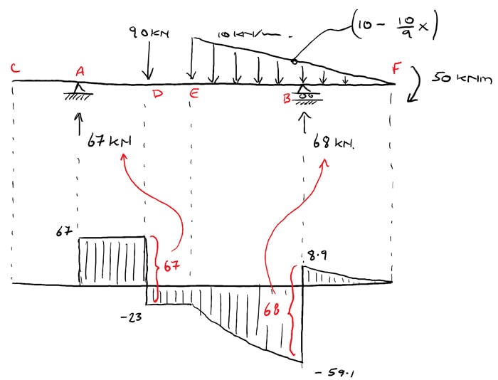
5.4 Cartoon the angle moment diagram

Once we've completed the shear force diagram, the bending moment diagram becomes much easier to determine. This is considering we tin can brand use of the following relationship between the shear force $V$ and the slope of the bending moment diagram,

(26) $\begin{equation*} \frac{\mathrm{d}M}{\mathrm{d}x} = V \end{equation*}$

Similarly to equation (23), this expressions allows us to infer a qualitative shape for the bending moment diagram, based on the shear strength diagram we've already calculated.

Consider the shear strength between A and D for case; it's abiding, which ways the slope of the bending moment diagram is likewise constant (an inclined directly line). Between D and E, the shear force is still abiding but has changed sign. This tells us the slope of the angle moment diagram has also changed sign, i.e. the bending moment diagram has a local elevation at D.

The fact that the shear strength is a polynomial (curve) between E and F also tells the states the angle moment's slope is continuously changing, i.e. it's also a curve. But the fact that the shear force changes sign at B, means the bending moment diagram has a peak at that point.

Finally, the externally applied moment at F tells united states that the bending moment diagram at this location has a value of $50\text{kNm}$ . Nosotros can combine all this information together to sketch out a qualitative bending moment diagram, based purely on the data encoded in the shear force diagram.

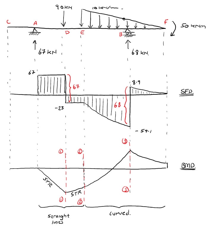
Shear-and-moment-diagrams-example-BMD-qualitative| DegreeTutors.com

Now we just have to cut the structure at detached locations (indicated with blood-red dashed lines above) to establish the various key values required to quantitatively ascertain the bending moment diagram. In this instance three cuts are sufficient:

at D to determine the local peak – Cut 1-1
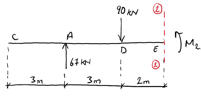
at E to determine the value on the boundary betwixt the straight and curved sections of the bending moment diagram – Cut 2-ii
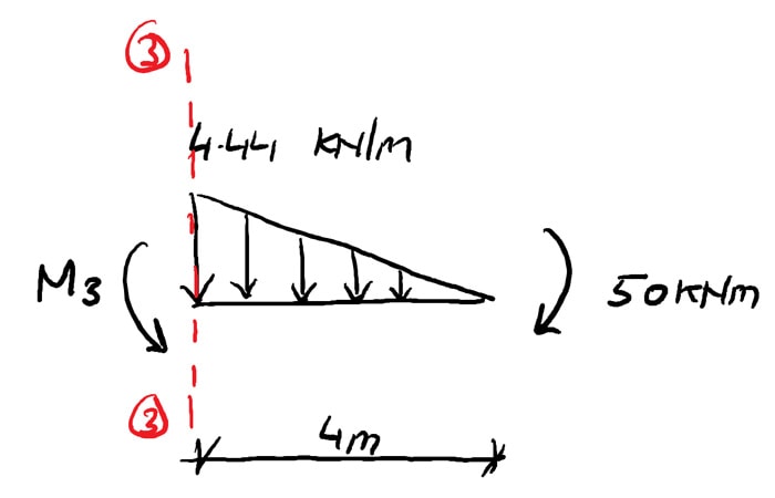
at B to determine the local peak – Cut 3-3

Cutting 1-i

As we've seen above, to make up one's mind the internal bending moment at D, $M_D$ , we cutting the structure to reveal the internal bending moment at this bespeak. And then by because moment equilibrium of the sub-construction we can solve for the value of $M_D$ .

Shear-and-moment-diagrams-example-Cut-1| DegreeTutors.com

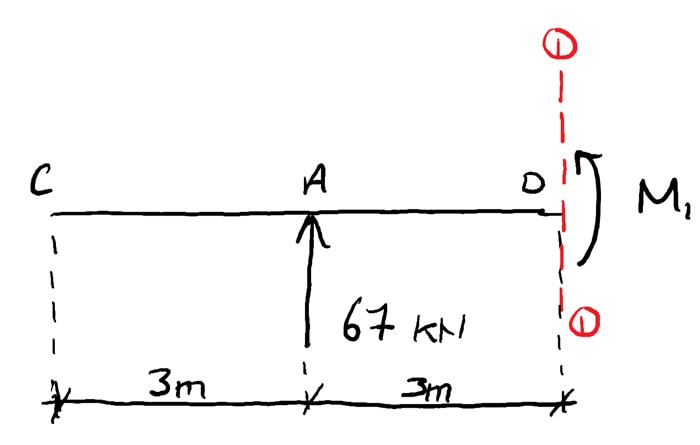
Taking the sum of the moments about the cutting,

(27) $\begin{equation*} \sum M_{\text{cut 1}}=0\:\:\text{(assume clockwise positive)} \end{equation*}$

(28) $\begin{equation*} -M_1 + (67\text{kN}\times 3\text{m}) = 0 \end{equation*}$

(29) $\begin{equation*} M_1 = 201\text{kNm} \end{equation*}$

Cut 2-2

Repeating this process for cut 2-two,

Shear-and-moment-diagrams-example-Cut-2| DegreeTutors.com

(thirty) $\begin{equation*} \sum M_{\text{cut 2}}=0\:\:\text{(assume clockwise positive)} \end{equation*}$

(31) $\begin{equation*} -M_2 + (67\text{kN}\times 5\text{m}) - (90\text{kN/m}\times 2\text{m}) = 0 \end{equation*}$

(32) $\begin{equation*} M_2 = 155\text{kNm} \end{equation*}$

Cutting 3-3

And finally for cut 3-three, this time considering equilibrium of the sub-structure to the right-hand side of the cutting

Shear-and-moment-diagrams-example-Cut-3| DegreeTutors.com

(33) $\begin{equation*} \sum M_{\text{cut 3}}=0\:\:\text{(assume clockwise positive)} \end{equation*}$

(34) $\begin{equation*} -M_3 + 50\text{kNm} + (4.44\text{kN/m}\times 4\text{m}\times 0.5 \times (4/3)\text{m}) = 0 \end{equation*}$

(35) $\begin{equation*} M_3 = 61.84\text{kNm} \end{equation*}$

We can at present sketch the complete quantitative bending moment diagram for the construction. In fact at this indicate we tin summarise the output of our consummate structural assay.

Shear-and-moment-diagrams-example-Summary-sketch| DegreeTutors.com

After working through this example, you might be interesting in this post, where we work through building a shear force and bending moment reckoner using Python. We actually build our calculator around this example question – so definitely worth a read when you finish up with this post.

half dozen.0 Relating Loading, Shear Force and Bending Moment

In the previous example, nosotros fabricated use of two very helpful differential relationships that related loading with shear force and shear force with angle moment. All the same we didn't properly introduce them. At present that we have a good idea of the general workflow for generating shear and moment diagrams, we can dig a chip deeper into these differential relationships. Understanding these, is the key to being able to build shear force and angle moment diagrams quickly and reliably.

Fully agreement the relationships we derive next will allow you to more 'intuitively excerpt' qualitative shear and moment diagrams 'by eye', with cuts used to confirm numerical values at salient points. Nosotros're going to explore 3 cases:

Case one: Uniformly distributed loading
Case 2: Signal force loading
Case 3: Indicate moment loading

In each example, our objective is to determine the relationship between the applied loading and the shear strength and bending moment information technology induces.

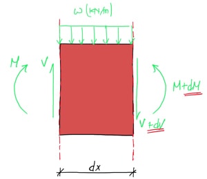
6.one Case 1: Uniformly distributed loading

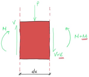
Consider a short segment of length $\mathrm{d}x$ cut from a axle and subject area to a uniformly distributed load with intensity $w$ kN/k. As nosotros saw above, these cuts have revealed the internal moment and shear on either side of the segment. Note the infinitesimal increase in moment ( $\mathrm{d}M$ ) and shear ( $\mathrm{d}V$ ) on the right side of the cut.

Beam segment with UDL | DegreeTutors.com

Shear Force

We tin can beginning by considering vertical force equilibrium for the segment. Since it must be in a state of static equilibrium, the sum of the vertical forces must equal zippo.

$\begin{equation*}\sum F_y = 0\:\:(\uparrow+ve)\end{equation*}$

$\begin{equation*}V-(v+\mathrm{d}V)-w\mathrm{d}x=0\end{equation*}$

(36) $\begin{equation*}\therefore \boxed{ \frac{\mathrm{d}V}{\mathrm{d}x} = -w}\end{equation*}$

In other words, the slope of the shear forcefulness diagram $(\mathrm{d}V/\mathrm{d}x)$ at a point is equal to the negative of the load intensity at that point. We tin can demonstrate this with a simple instance. Consider the beam below subject to a distributed load with linearly increasing intensity. By making a cut at a distance $x$ from the left support with reveal the internal shear force $V(x)$ .

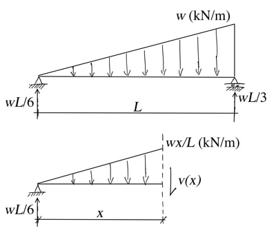
If the load intensity increases linearly from zippo to $w$ , then at the cut the load intensity is $wx/L$ . We tin now evaluate vertical force equilibrium for the sub-structure,

$\begin{equation*}\sum F_y = 0\:\:(\uparrow+ve)\end{equation*}$

$\begin{equation*}V(x) = \frac{wl}{6} - \frac{wx^2}{2L}\end{equation*}$

Nosotros can now differentiate the expression for $V(x)$ yielding,

$\begin{equation*}\frac{\mathrm{d}V}{\mathrm{d}x} = -\frac{wx}{L}\end{equation*}$

So we tin can encounter that the differential of the shear force is equal to the negative of the load intensity. It'south also worth noting the shape of the SFD, pictured beneath. At the left mitt support when the load intensity is nothing, the SFD has a value of $wL/6$ (the value of the left reaction) simply it is horizontal, i.e. has a slope of zero. As the load intensity increases equally we move from left to right, the SFD gets steeper. i.eastward. the slope increases.

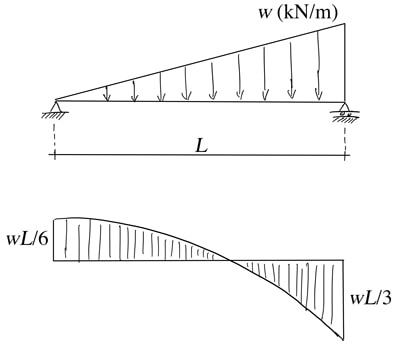
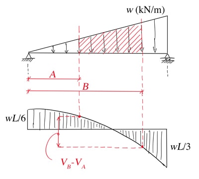
Another implication of this differential human relationship between shear force and load intensity tin be seen if we integrate both sides of the equation,

$\begin{equation*}\frac{\mathrm{d}V}{\mathrm{d}x} = -w\end{equation*}$

$\begin{equation*}\int_A^B \mathrm{d}V = -\int_A^B w\: \mathrm{d}x\end{equation*}$

(37) $\begin{align*}V_B - V_A &= -\int_A^B w\: \mathrm{d}x\\&= - \:\text{area under loading diagram between A and B}\end{align*}$

We can come across this represented graphically in the image below.

Bending Moment

Having established the key relationship for shear, at present we can turn our attention to angle moments. Referring back to our beam segment of length $\mathrm{d}x$ and considering moment equilibrium of the segment by taking moments about the left paw side of the segment,

$\begin{equation*}\sum M_{\text{LHS}} = 0 \:\:(\curvearrowright +ve)\end{equation*}$

$\begin{equation*}M-(M+\mathrm{d}M)+(V+\mathrm{d}V)(\mathrm{d}x)+w. \mathrm{d}x. \frac{\mathrm{d}x}{2} = 0\end{equation*}$

(38) $\begin{equation*}\therefore \boxed{ \frac{\mathrm{d}M}{\mathrm{d}x} = V}\end{equation*}$

And then, the slope of the BMD at a point equals the shear force at that point. Combined with the previous differential equation we derived, this is a very helpful equation. Whenever nosotros have a beam subject to a distributed load, we can use these equations to infer the shape of the SFD and BMD. Consider the SFD and BMD for our beam below.

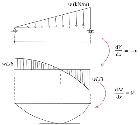
We annotation that when the shear force is null, the gradient of the BMD is also cypher indicating a local maximum in the BMD. We also annotation the modify in sign of the slope of the BMD as the shear force goes from positive to negative. Remember that the shape of the SFD was itself deduced from the shape of the loading diagram. By making use of these relationships between loading, SFD and BMD, we can build upward a qualitative picture show of structural behaviour.

6.2 Example 2: Point strength loading

At present we echo the aforementioned procedure as above merely this time our beam segment is subject to a point load $P$ located at $\mathrm{d}x/2$ . Annotation that on the right hand side of the element, the internal shear force and angle moment have increased by a finite amount rather than an minute corporeality as was the case previously.

Beam segment with point loading | DegreeTutors.com

Shear Forcefulness

Evaluating the sum of the vertical forces yields,

$\begin{equation*}\sum F_y = 0\:\:(\uparrow+ve)\end{equation*}$

$\begin{equation*}-P +V - (V+V_1)=0\end{equation*}$

(39) $\begin{equation*}\therefore \boxed{ V_1 = -P_1 }\end{equation*}$

From this nosotros see that a signal load induces a footstep change in the SFD. We've already seen this when nosotros followed the loads across the construction to build the shear force diagram above. This equation is simply the mathematical representation of this. Consider for example the simple case below of a beam subject to 2 point loads.

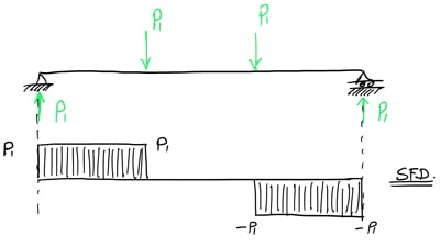
Beam with two point loads | DegreeTutors.com

Nosotros can readily see the step changes in the shear forcefulness diagram existence equal to the magnitude of the indicate loads at that location.

Bending Moment

If we now consider moment equilibrium of our segment,

$\begin{equation*}\sum M_{\text{LHS}} = 0 \:\:(\curvearrowright +ve)\end{equation*}$

$\begin{equation*}M-(M+M_1) + P\frac{\mathrm{d}x}{2} + (V+V_1)\mathrm{d}x\end{equation*}$

$\begin{equation*}M_1 = \underbrace{P\frac{\mathrm{d}x}{2} + (V+V_1)\mathrm{d}x}_{\text{infinitesimally small}}\end{equation*}$

$\begin{equation*}\therefore \boxed{M_1 \approx 0}\end{equation*}$

The presence of infinitesimally small segment lengths on the right hand side of the equal sign ways that $M_1$ is infinitesimally minor. From this we conclude that the presence of a point load does not change the value of the angle moment diagram at a bespeak.

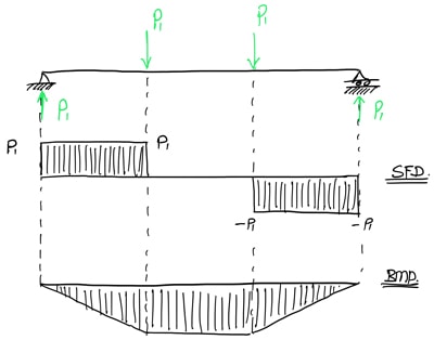
Even so, noting that the shear force changes from $V$ to $V-P$ , we tin can say, according to the expression,

(twoscore) $\begin{equation*}\frac{\mathrm{d}M}{\mathrm{d}x} = V\end{equation*}$

that the gradient of the bending moment diagram changes by an amount $P$ . Once again, we can meet how this maps onto our uncomplicated example below. Note that at the betoken of awarding of $P_1$ , the slope of the bending moment diagram changes. Too, where the shear strength is aught, the bending moment diagram is horizontal.

So we have added 2 more than equations into our toolbox for establishing qualitative structural behaviour.

Beam with two point loads and diagrams | DegreeTutors.com

6.3 Case 3: Point moment loading

Finally we tin repeat the analysis for the instance of moment applied at a bespeak.

Beam segment with point moment | DegreeTutors.com

Shear Force

Have the sum of the forces in the vertical direction,

$\begin{equation*}\sum F_y = 0\:\:(\uparrow+ve)\end{equation*}$

$\begin{equation*}V-(V+V_1)\end{equation*}$

$\begin{equation*}\therefore \boxed{V_1 = 0}\end{equation*}$

And then, the shear force diagram does not change with the application of a moment.

Bending Moment

Taking the sum of the moments nearly the left hand side of the cut,

$\begin{equation*}\sum M_{\text{LHS}} = 0 \:\:(\curvearrowright +ve)\end{equation*}$

$\begin{equation*}M+M_o-(M+M_1)+\underbrace{(V+V_1)\mathrm{d}x}_{\text{infinitesimally small}\rightarrow 0} = 0\end{equation*}$

$\begin{equation*}\therefore \boxed{M_0 = M_1}\end{equation*}$

This means that at the signal of application of a angle moment, at that place is a step change in the bending moment diagram, equal to the magnitude of the moment practical.

The 6 boxed equations in this section higher up can be used to infer a huge amount of data about the behaviour of a structure under load. Let'south put this into practise with some other worked instance.

7.0 Some other Instance

Determine the shear strength diagram and angle moment diagram for the post-obit simply supported beam. Make certain to attempt this yourself before watching the solution videos.

Shear and moment example | DegreeTutors.com

seven.1 Setup and shear force diagram

7.two Building the bending moment diagram

7.3 Confirming maximum moment with calculus

So there you have it. Nosotros've linked together the internal normal and shear stresses with the bending moment and shear force diagrams. And nosotros've derived a toolbox full of helpful differential equations to help us quickly and intuitively build shear force and bending moment diagrams. There is quite a lot more than we could say about shear and moment diagrams. Simply that's probably enough for one post.

The best way for you to go amend at evaluating shear force and bending moment diagrams is through do. There actually are no shortcuts I'k afraid. The proficient news is, the more you practise, the quicker you get and the stronger your intuition for structural behaviour becomes. That's all for now, I hope you got some value from reading this mail service and I'll see y'all in the next one.

Build your ain shear force and bending moment solver

Understanding how to build shear force and bending moment diagrams the way we've demonstrated in a higher place is an essential skill. Even so, the process is time consuming, particularly when you enter the iterative process of analysis and design. And that'southward earlier we fifty-fifty kickoff talking about how to handle indeterminate structures! For these reasons, we generally make use of structural analysis software to speed the procedure upwardly. But this software is typically expensive and for the vast majority of cases, has way more functionality than we need. And then – why not just build you own, for (almost) free! In my course beneath, we use the Direct Stiffness Method to build our own 2D beam and frame analysis programme using Python. Y'all don't need to be a programmer to have this course. When you're finished it…you'll accept your own DIY structural assay programme.

Source: https://www.degreetutors.com/shear-and-moment-diagrams/

Posted by: holcombworeuthe93.blogspot.com

How To Draw Shear Stress Distribution Diagram

Shear and Moment Diagrams – An Ultimate Guide

one.0 What is a Bending Moment?

2.0 What is a Shear Forcefulness?

three.0 Calculating Internal Shear Forces and Angle Moments

4.0 Building Shear and Moment Diagrams

4.1 Finding the location of the maximum bending moment

5.0 Drawing Shear Strength and Bending Moment Diagrams – An Instance

5.1 Video Tutorial

5.2 Computing the support reactions

v.three Drawing the shear force diagram

5.4 Cartoon the angle moment diagram

half dozen.0 Relating Loading, Shear Force and Bending Moment

6.one Case 1: Uniformly distributed loading

6.2 Example 2: Point strength loading

6.3 Case 3: Point moment loading

7.0 Some other Instance

seven.1 Setup and shear force diagram

7.two Building the bending moment diagram

7.3 Confirming maximum moment with calculus

Build your ain shear force and bending moment solver

0 Response to "How To Draw Shear Stress Distribution Diagram"

Post a Comment

Iklan Atas Artikel

Iklan Tengah Artikel 1

Iklan Tengah Artikel 2

Iklan Bawah Artikel